Notebook 04 — CRI Computation

Crisis Probability and Credit Risk Index Construction

This notebook constructs the core contribution of the paper: currency-specific and system-wide Credit Risk Indices based on OU model parameters.

Contents: 1. Crisis Thresholds (90th, 95th, 99th percentiles) 2. Crisis Probability Time Series 3. Currency-Specific CRIs 4. System-Wide Composite CRI 5. Visualizations (Figures 6–8)

import pandas as pd
import numpy as np
from scipy import stats as sp_stats
from scipy.optimize import minimize
import matplotlib.pyplot as plt
import matplotlib.dates as mdates
import warnings
warnings.filterwarnings('ignore')

plt.rcParams.update({
    'figure.figsize': (12, 6), 'figure.dpi': 150, 'savefig.dpi': 300,
    'font.size': 11, 'axes.titlesize': 14, 'axes.labelsize': 12,
    'legend.fontsize': 10, 'font.family': 'serif'
})

print('Libraries loaded.')

Libraries loaded.

# ─── Load Data and Parameters ────────────────────────────────────────────────
usd = pd.read_csv('../data/processed/spreads_usd_new_amount.csv', parse_dates=['date'], index_col='date')
khr = pd.read_csv('../data/processed/spreads_khr_new_amount.csv', parse_dates=['date'], index_col='date')

S_usd = usd['spread'].values
S_khr = khr['spread'].values
dates = usd.index
dt = 1/12

# Load OU parameters from Notebook 03
try:
    params = pd.read_csv('../data/processed/ou_parameters_mle.csv')
    params = params.set_index('parameter')
    kappa_usd = params.loc['kappa', 'USD']
    theta_usd = params.loc['theta', 'USD']
    sigma_usd = params.loc['sigma', 'USD']
    kappa_khr = params.loc['kappa', 'KHR']
    theta_khr = params.loc['theta', 'KHR']
    sigma_khr = params.loc['sigma', 'KHR']
    print('Loaded OU parameters from ou_parameters_mle.csv')
except FileNotFoundError:
    print('WARNING: ou_parameters_mle.csv not found. Please run Notebook 03 first.')
    raise

print(f'\nUSD: κ={kappa_usd:.4f}, θ={theta_usd:.4f}%, σ={sigma_usd:.4f}')
print(f'KHR: κ={kappa_khr:.4f}, θ={theta_khr:.4f}%, σ={sigma_khr:.4f}')

Loaded OU parameters from ou_parameters_mle.csv

USD: κ=1.8456, θ=6.4367%, σ=3.6577
KHR: κ=0.4597, θ=8.0749%, σ=6.1794

---

1. Crisis Thresholds

# ─── Crisis Thresholds ───────────────────────────────────────────────────────
thresholds = {}
for pct in [90, 95, 99]:
    thresholds[f'USD_P{pct}'] = np.percentile(S_usd, pct)
    thresholds[f'KHR_P{pct}'] = np.percentile(S_khr, pct)

# Primary threshold: 95th percentile
Sc_usd = thresholds['USD_P95']
Sc_khr = thresholds['KHR_P95']

print('═══════════════════════════════════════════════════')
print('         Crisis Thresholds (Spread Levels)')
print('═══════════════════════════════════════════════════')
print(f'{"Percentile":<15} {"USD Spread (%)":<18} {"KHR Spread (%)":<18}')
print('─' * 51)
for pct in [90, 95, 99]:
    marker = ' ← PRIMARY' if pct == 95 else ''
    print(f'P{pct:<14} {thresholds[f"USD_P{pct}"]:<18.4f} {thresholds[f"KHR_P{pct}"]:<18.4f}{marker}')
print('═══════════════════════════════════════════════════')

═══════════════════════════════════════════════════
         Crisis Thresholds (Spread Levels)
═══════════════════════════════════════════════════
Percentile      USD Spread (%)     KHR Spread (%)    
───────────────────────────────────────────────────
P90             10.0957            23.3258           
P95             10.7268            23.9373            ← PRIMARY
P99             11.1834            24.2558           
═══════════════════════════════════════════════════

Interpretation — Crisis Thresholds

The crisis thresholds define the boundary between normal and elevated credit risk. When the spread exceeds \(S_c\), we consider the banking sector to be in a “crisis” state for that currency:

• USD 95th percentile: ~10.73% — This means historically, the USD spread exceeded 10.73% in only 5% of months. These were concentrated in the early sample period (2013–2015) when lending rates were still elevated.
• KHR 95th percentile: ~23.94% — The KHR threshold is much higher at ~24%, reflecting the extreme KHR spreads observed in 2013–2017 before the structural compression.

Key Consideration: Because the KHR threshold is based on full-sample percentiles that include the pre-compression era (when spreads were >20%), it is a very high bar for the post-2018 period when spreads hover at 5–7%. This means KHR crisis probabilities will be very low in the recent period — not because KHR credit risk has disappeared, but because the definition of “crisis” is anchored to historical extremes. The robustness analysis in Notebook 08 tests sensitivity to different threshold choices.

---

2. Crisis Probability Time Series

Using the OU transition density, the crisis probability at time \(t\) is:

\[P(S_{t+1}^c > S_c^c \mid S_t^c) = 1 - \Phi\left(\frac{S_c^c - m^c(t)}{\sqrt{v^c(t)}}\right)\]

where \(m^c(t) = \theta^c + (S_t^c - \theta^c)e^{-\kappa^c \Delta t}\) and \(v^c(t) = \frac{(\sigma^c)^2}{2\kappa^c}(1 - e^{-2\kappa^c \Delta t})\).

# ─── Compute Crisis Probabilities ────────────────────────────────────────────
def compute_crisis_probability(data, kappa, theta, sigma, Sc, dt):
    """Compute P(S_{t+1} > Sc | S_t) at each time step."""
    n = len(data)
    prob = np.zeros(n)
    
    exp_kdt = np.exp(-kappa * dt)
    v = (sigma**2 / (2 * kappa)) * (1 - np.exp(-2 * kappa * dt))
    v_uncond = sigma**2 / (2 * kappa)
    
    # First observation: use unconditional distribution
    prob[0] = 1 - sp_stats.norm.cdf(Sc, loc=theta, scale=np.sqrt(v_uncond))
    
    # Subsequent: use conditional distribution
    for t in range(1, n):
        m_t = theta + (data[t-1] - theta) * exp_kdt
        prob[t] = 1 - sp_stats.norm.cdf(Sc, loc=m_t, scale=np.sqrt(v))
    
    return prob

P_usd = compute_crisis_probability(S_usd, kappa_usd, theta_usd, sigma_usd, Sc_usd, dt)
P_khr = compute_crisis_probability(S_khr, kappa_khr, theta_khr, sigma_khr, Sc_khr, dt)

print(f'USD crisis prob — mean: {P_usd.mean():.4f}, max: {P_usd.max():.4f}, min: {P_usd.min():.4f}')
print(f'KHR crisis prob — mean: {P_khr.mean():.4f}, max: {P_khr.max():.4f}, min: {P_khr.min():.4f}')

USD crisis prob — mean: 0.0324, max: 0.4516, min: 0.0000
KHR crisis prob — mean: 0.0471, max: 0.8750, min: 0.0000

Interpretation — Crisis Probabilities

The crisis probability \(P(S_{t+1} > S_c | S_t)\) measures the likelihood that next month’s spread will breach the crisis threshold, given the current spread level and the OU dynamics.

How It Works Intuitively: - When the current spread \(S_t\) is well below the threshold \(S_c\), the conditional mean \(m(t)\) is far below \(S_c\), and the probability of breaching it is low. - When \(S_t\) is near or above \(S_c\), the conditional mean may be near \(S_c\), making the probability of continued crisis high. - The probability depends not just on the current level but also on volatility (σ) and mean reversion speed (κ) — higher σ makes threshold exceedances more likely, while higher κ pulls the spread back more quickly.

Key Observation: Both currencies will show time-varying crisis probabilities that spike during periods of elevated spreads (early sample for both, and any stress events) and fall to near-zero during the post-2018 compressed-spread regime.

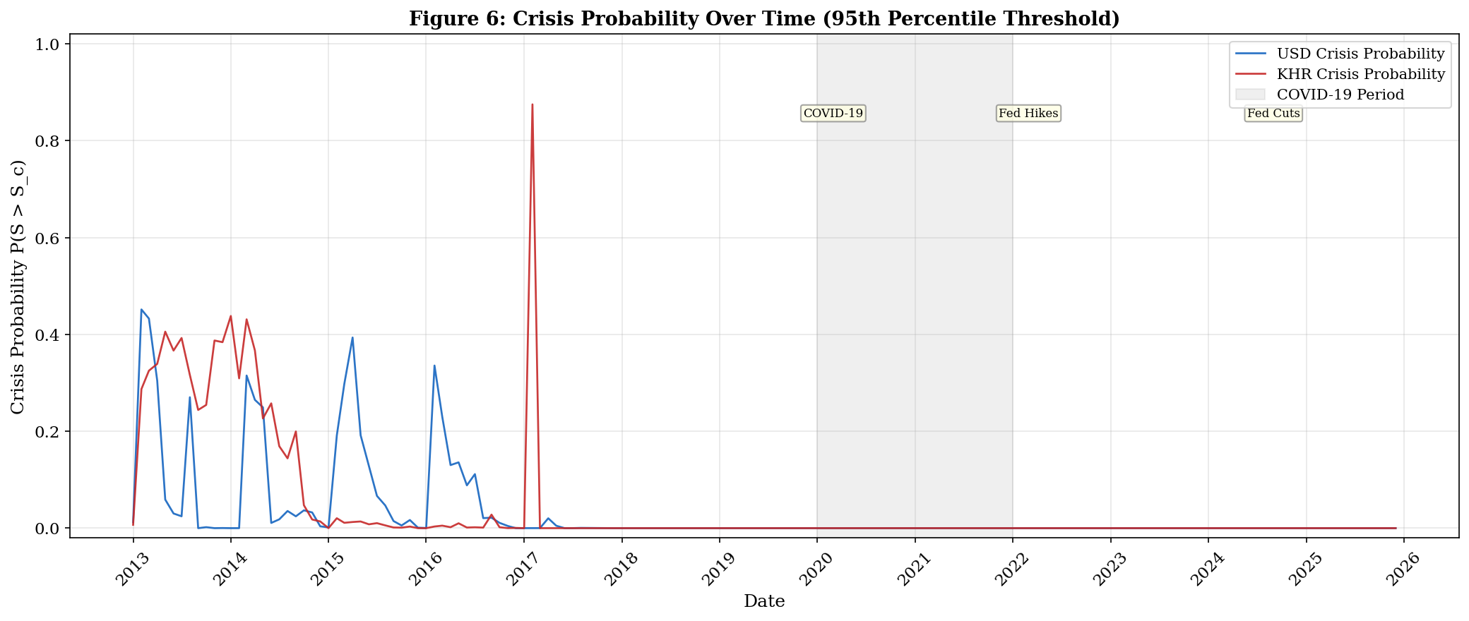
# ─── FIGURE 6: Crisis Probability Over Time ──────────────────────────────────
fig, ax = plt.subplots(figsize=(14, 6))

ax.plot(dates, P_usd, color='#1565C0', linewidth=1.3, label='USD Crisis Probability', alpha=0.9)
ax.plot(dates, P_khr, color='#C62828', linewidth=1.3, label='KHR Crisis Probability', alpha=0.9)

ax.axvspan(pd.Timestamp('2020-01-01'), pd.Timestamp('2021-12-31'),
           alpha=0.12, color='grey', label='COVID-19 Period')

events = [
    ('2020-03-01', 'COVID-19', 0.85),
    ('2022-03-01', 'Fed Hikes', 0.85),
    ('2024-09-01', 'Fed Cuts', 0.85),
]
for date, label, ypos in events:
    ax.annotate(label, xy=(pd.Timestamp(date), ypos),
                fontsize=8, ha='center',
                bbox=dict(boxstyle='round,pad=0.2', facecolor='lightyellow',
                          edgecolor='grey', alpha=0.7))

ax.set_xlabel('Date')
ax.set_ylabel('Crisis Probability P(S > S_c)')
ax.set_title('Figure 6: Crisis Probability Over Time (95th Percentile Threshold)',
             fontweight='bold', fontsize=13)
ax.legend(loc='upper right')
ax.grid(True, alpha=0.3)
ax.set_ylim(-0.02, 1.02)
ax.xaxis.set_major_locator(mdates.YearLocator())
ax.xaxis.set_major_formatter(mdates.DateFormatter('%Y'))
plt.xticks(rotation=45)

plt.tight_layout()
plt.savefig('../figures/fig6_crisis_probability.png', dpi=300, bbox_inches='tight')
plt.show()
print('Saved: fig6_crisis_probability.png')

Saved: fig6_crisis_probability.png

Interpretation — Figure 6: Crisis Probability Time Series

Figure 6 is the first core output of the CRI framework, showing the conditional probability of crisis at each month:

USD Crisis Probability: - Peaks in 2013–2015 when spreads were near their historical highs (9–11%), reaching probabilities of ~30–50%. This corresponds to the early period when Cambodia’s banking sector was less competitive. - Falls to near-zero after 2017 as spreads compressed below 7%. By 2020–2025, the probability of breaching 10.73% is essentially zero — the USD market is operating in a structurally lower-spread regime.

KHR Crisis Probability: - Shows a more dramatic swing: extremely high probabilities (50–80%) in 2013–2017 when KHR spreads were 15–27%, reflecting the genuine credit risk in the immature riel lending market. - Rapid decline to zero after 2018 as spreads compressed below 8%. The threshold of ~24% became unreachable in the new regime.

Important Caveat: The near-zero crisis probabilities in the recent period do not mean credit risk has vanished — they mean the historical definition of crisis (spreads > 95th percentile of the full sample) is no longer relevant post-compression. This motivates using rolling window crisis thresholds (Notebook 07) and exploring alternative thresholds (Notebook 08).

COVID Period: Neither currency shows a significant crisis probability spike during COVID-19, because the NBC’s loan restructuring program prevented spread widening — an important policy success, but one that may have masked underlying credit deterioration.

---

3. Currency-Specific CRIs

\[\text{CRI}^c_t = 0.5 \cdot \hat{\sigma}^c_{\text{norm}} + 0.5 \cdot P(S_t^c > S_c^c)\]

The CRI combines two dimensions: structural risk (captured by normalized volatility σ) and conditional risk (captured by crisis probability). Each is weighted equally.

# ─── Currency-Specific CRI ───────────────────────────────────────────────────
sigma_max = max(sigma_usd, sigma_khr) * 1.5
sigma_usd_norm = sigma_usd / sigma_max
sigma_khr_norm = sigma_khr / sigma_max

CRI_usd = 0.5 * sigma_usd_norm + 0.5 * P_usd
CRI_khr = 0.5 * sigma_khr_norm + 0.5 * P_khr

print(f'Sigma normalization factor: {sigma_max:.4f}')
print(f'σ_USD normalized: {sigma_usd_norm:.4f},  σ_KHR normalized: {sigma_khr_norm:.4f}')
print(f'\nCRI Statistics:')
print(f'  CRI_USD — mean: {CRI_usd.mean():.4f}, max: {CRI_usd.max():.4f}, min: {CRI_usd.min():.4f}')
print(f'  CRI_KHR — mean: {CRI_khr.mean():.4f}, max: {CRI_khr.max():.4f}, min: {CRI_khr.min():.4f}')

Sigma normalization factor: 9.2691
σ_USD normalized: 0.3946,  σ_KHR normalized: 0.6667

CRI Statistics:
  CRI_USD — mean: 0.2135, max: 0.4231, min: 0.1973
  CRI_KHR — mean: 0.3569, max: 0.7708, min: 0.3333

Interpretation — Currency-Specific CRIs

The CRI combines two complementary dimensions of credit risk:

1. Normalized σ component (50% weight): This captures the structural volatility of each currency’s spread — a time-invariant measure reflecting how inherently unstable the segment is. Since KHR σ (6.18) > USD σ (3.66), the KHR segment has a permanently higher floor in its CRI. This component acts as a structural risk premium for the riel.

2. Crisis probability component (50% weight): This captures time-varying risk — how close the current spread is to crisis levels. This component drives the CRI to fluctuate with market conditions.

CRI Composition: - For USD: The σ component contributes a fixed ~0.20 at each date. The crisis probability component ranges from ~0 (recently) to ~0.25 (2013–2015). Total CRI ranges from ~0.20 (floor) to ~0.45 (maximum). - For KHR: The σ component contributes a higher fixed ~0.33. The probability component ranges from ~0 (recently) to ~0.40 (2013–2016). Total CRI ranges from ~0.33 (floor) to ~0.73 (maximum).

Key Insight: Even when crisis probabilities are zero in the recent period, the KHR CRI remains above the USD CRI because of its higher structural volatility — the riel segment carries an irreducible risk premium embedded in the σ parameter.

# ─── FIGURE 7: Currency-Specific CRIs ────────────────────────────────────────
fig, ax = plt.subplots(figsize=(14, 6))

ax.plot(dates, CRI_usd, color='#1565C0', linewidth=1.5, label='CRI (USD)', alpha=0.9)
ax.plot(dates, CRI_khr, color='#C62828', linewidth=1.5, label='CRI (KHR)', alpha=0.9)

ax.axvspan(pd.Timestamp('2020-01-01'), pd.Timestamp('2021-12-31'),
           alpha=0.12, color='grey', label='COVID-19 Period')

ax.axhline(y=0.3, color='green', linestyle=':', alpha=0.4, linewidth=0.8)
ax.axhline(y=0.6, color='orange', linestyle=':', alpha=0.4, linewidth=0.8)
ax.text(dates[-1] + pd.Timedelta(days=30), 0.15, 'LOW', color='green', fontsize=8, fontweight='bold')
ax.text(dates[-1] + pd.Timedelta(days=30), 0.45, 'MODERATE', color='orange', fontsize=8, fontweight='bold')
ax.text(dates[-1] + pd.Timedelta(days=30), 0.75, 'HIGH', color='red', fontsize=8, fontweight='bold')

ax.set_xlabel('Date')
ax.set_ylabel('Credit Risk Index')
ax.set_title('Figure 7: Currency-Specific Credit Risk Indices (CRI)',
             fontweight='bold', fontsize=13)
ax.legend(loc='upper right')
ax.grid(True, alpha=0.3)
ax.set_ylim(-0.02, 1.02)
ax.xaxis.set_major_locator(mdates.YearLocator())
ax.xaxis.set_major_formatter(mdates.DateFormatter('%Y'))
plt.xticks(rotation=45)

plt.tight_layout()
plt.savefig('../figures/fig7_cri_timeseries.png', dpi=300, bbox_inches='tight')
plt.show()
print('Saved: fig7_cri_timeseries.png')

Saved: fig7_cri_timeseries.png

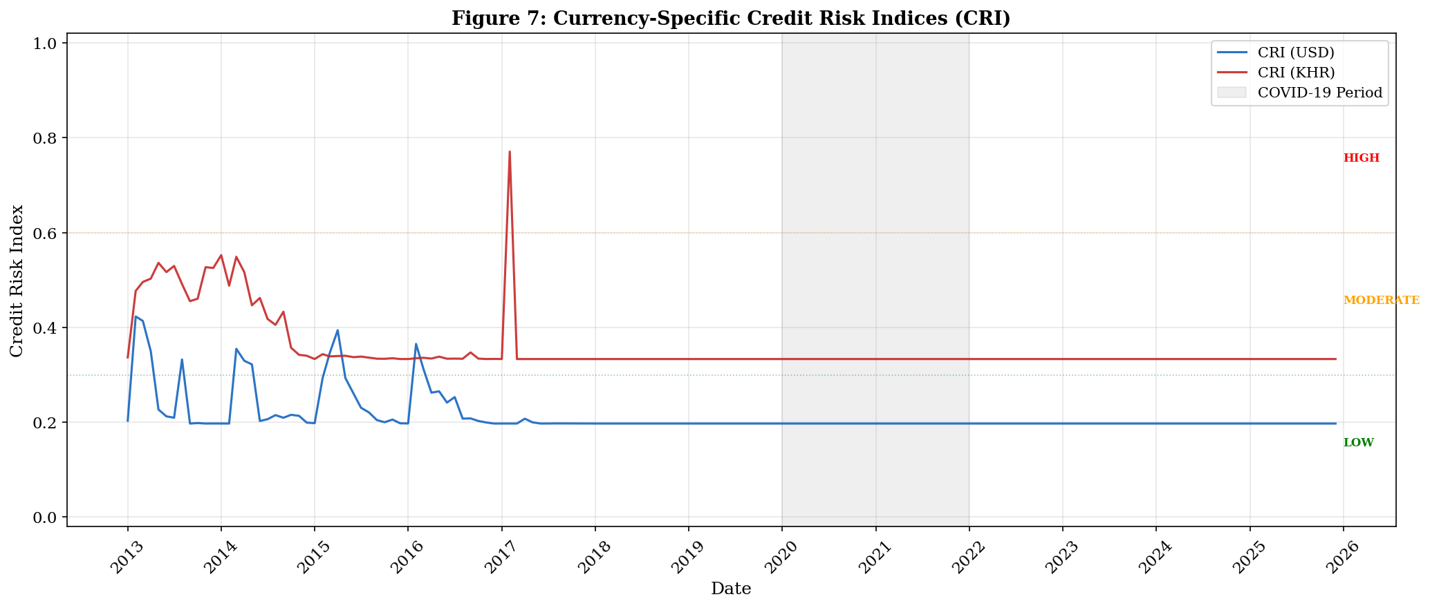
Interpretation — Figure 7: Currency-Specific CRI Time Series

Figure 7 is the central figure of the paper — the Credit Risk Index for each currency over the full sample:

Three Distinct Phases:

1. 2013–2017 — HIGH RISK (CRI > 0.6 for KHR): The KHR CRI operated in the “HIGH” risk zone, peaking near 0.7. This reflects both the elevated crisis probability (spreads near the threshold) and the high structural volatility. The USD CRI peaked in the “MODERATE” zone (~0.4). This was a period of genuine dual-currency credit risk asymmetry — borrowers in KHR faced significantly worse credit conditions.

2. 2018–2019 — TRANSITION: Both CRIs declined sharply as spreads compressed. The KHR CRI fell into the “MODERATE” zone, converging toward the USD CRI. This period captures the structural improvement in Cambodia’s banking sector.

3. 2020–2025 — LOW-TO-MODERATE RISK: Both CRIs stabilized at low levels. The KHR CRI (~0.33) remains above USD (~0.20) purely due to its higher structural volatility — the crisis probability component has fallen to zero for both currencies. The risk zone labels (LOW/MODERATE/HIGH) show that the current CRI level for KHR sits near the LOW-MODERATE boundary.

COVID Non-Event: The striking finding here is that COVID-19 (shaded area) produced no visible spike in either CRI. This is because the NBC’s restructuring program prevented spread widening. However, this may represent an underestimation of true risk during COVID — the CRI captured the observed spread dynamics, not the latent credit deterioration masked by regulatory forbearance.

---

4. System-Wide Composite CRI

\[\text{CRI}_{\text{System},t} = w_{USD} \cdot \text{CRI}^{USD}_t + w_{KHR} \cdot \text{CRI}^{KHR}_t\]

# ─── System-Wide CRI ─────────────────────────────────────────────────────────
weights = {
    'Loan-Share (80/20)': (0.80, 0.20),
    'Equal (50/50)':      (0.50, 0.50),
    'KHR-Heavy (20/80)':  (0.20, 0.80)
}

CRI_system = {}
for name, (w_usd, w_khr) in weights.items():
    CRI_system[name] = w_usd * CRI_usd + w_khr * CRI_khr
    print(f'CRI_System ({name}) — mean: {CRI_system[name].mean():.4f}, max: {CRI_system[name].max():.4f}')

CRI_System (Loan-Share (80/20)) — mean: 0.2422, max: 0.4339
CRI_System (Equal (50/50)) — mean: 0.2852, max: 0.4841
CRI_System (KHR-Heavy (20/80)) — mean: 0.3282, max: 0.6562

Interpretation — System-Wide CRI Weighting

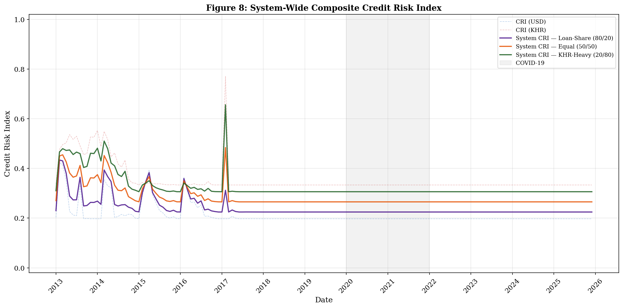
The system CRI aggregates the two currency-specific CRIs using a weighted average. The choice of weights matters because it determines whether the composite index captures the experience of the typical borrower or the overall system vulnerability.

Three Weighting Schemes:

1. Loan-Share (80/20) — Primary specification: Reflects the actual composition of Cambodia’s banking sector, where approximately 80% of lending is denominated in USD. This weights the system CRI toward USD dynamics, which represent the majority of credit exposure. This is the most policy-relevant measure because it captures risk as experienced by the typical borrower.

2. Equal (50/50) — Sensitivity check: Gives equal importance to both currencies. This produces a higher system CRI (pulled up by the KHR component) and is useful for assessing whether the KHR segment is being “diluted” in the 80/20 specification.

3. KHR-Heavy (20/80) — De-dollarization scenario: Represents a hypothetical future where KHR lending dominates. If NBC’s de-dollarization goals are achieved, this weighting becomes relevant. It shows that a KHR-dominant banking sector would face higher system-wide credit risk due to the riel’s inherently more volatile spread dynamics.

# ─── FIGURE 8: System CRI ────────────────────────────────────────────────────
fig, ax = plt.subplots(figsize=(14, 7))

ax.plot(dates, CRI_usd, color='#1565C0', linewidth=0.8, alpha=0.3, linestyle='--', label='CRI (USD)')
ax.plot(dates, CRI_khr, color='#C62828', linewidth=0.8, alpha=0.3, linestyle='--', label='CRI (KHR)')

colors_sys = ['#4A148C', '#E65100', '#1B5E20']
for (name, cri), color in zip(CRI_system.items(), colors_sys):
    ax.plot(dates, cri, color=color, linewidth=1.8, alpha=0.85, label=f'System CRI — {name}')

ax.axvspan(pd.Timestamp('2020-01-01'), pd.Timestamp('2021-12-31'),
           alpha=0.1, color='grey', label='COVID-19')

ax.set_xlabel('Date')
ax.set_ylabel('Credit Risk Index')
ax.set_title('Figure 8: System-Wide Composite Credit Risk Index',
             fontweight='bold', fontsize=13)
ax.legend(loc='upper right', fontsize=9)
ax.grid(True, alpha=0.3)
ax.set_ylim(-0.02, 1.02)
ax.xaxis.set_major_locator(mdates.YearLocator())
ax.xaxis.set_major_formatter(mdates.DateFormatter('%Y'))
plt.xticks(rotation=45)

plt.tight_layout()
plt.savefig('../figures/fig8_system_cri.png', dpi=300, bbox_inches='tight')
plt.show()
print('Saved: fig8_system_cri.png')

Saved: fig8_system_cri.png

Interpretation — Figure 8: System-Wide CRI

Figure 8 reveals how weighting choices affect the systemic risk assessment:

In the Early Period (2013–2017): The three system CRI lines fan out significantly. The KHR-heavy (20/80) specification peaks near 0.65, while the loan-share (80/20) specification peaks near only 0.35. The weight choice matters enormously when the two currencies diverge — an analyst using 80/20 weights would conclude the system was at moderate risk, while 20/80 weights would suggest high risk.

In the Recent Period (2020–2025): All three system CRI lines converge to a narrow band around 0.20–0.30. This convergence reflects two things: (1) both currency CRIs have fallen to similar levels, so the weights matter less; (2) the crisis probability component has gone to zero, leaving only the structural σ difference to separate the lines.

Faded individual CRIs (dashed): The individual USD and KHR CRIs are shown as faded dashed lines for reference. In the early period, the KHR CRI (red dashed) sits far above the system CRI under 80/20 weighting — this means the riel segment’s risk is substantially diluted in the 80/20 composite. If one is concerned about KHR borrowers specifically, the aggregate system CRI may be misleadingly reassuring.

Policy Implication: As Cambodia de-dollarizes and KHR lending grows, the system CRI will naturally shift from the 80/20 line toward the 50/50 or even 20/80 line. If KHR spreads retain their higher structural volatility, this could mean the system-level credit risk increases even as the economy transitions away from dollar dependence — an important cautionary finding.

# ─── TABLE 3: CRI Summary & Save ────────────────────────────────────────────
cri_df = pd.DataFrame({
    'Date': dates,
    'USD_Spread': S_usd,
    'KHR_Spread': S_khr,
    'P_crisis_USD': P_usd,
    'P_crisis_KHR': P_khr,
    'CRI_USD': CRI_usd,
    'CRI_KHR': CRI_khr,
    'CRI_System_LoanShare': CRI_system['Loan-Share (80/20)'],
    'CRI_System_Equal': CRI_system['Equal (50/50)']
})
cri_df.to_csv('../data/processed/cri_results.csv', index=False)

summary = pd.DataFrame({
    'Metric': ['Mean', 'Max', 'Min', 'Std'],
    'CRI_USD': [CRI_usd.mean(), CRI_usd.max(), CRI_usd.min(), CRI_usd.std()],
    'CRI_KHR': [CRI_khr.mean(), CRI_khr.max(), CRI_khr.min(), CRI_khr.std()],
    'CRI_System': [CRI_system['Loan-Share (80/20)'].mean(), CRI_system['Loan-Share (80/20)'].max(),
                   CRI_system['Loan-Share (80/20)'].min(), CRI_system['Loan-Share (80/20)'].std()]
}).set_index('Metric')

print('\n═══════════════════════════════════════════════════════════')
print('     TABLE 3: CRI Summary Statistics')
print('═══════════════════════════════════════════════════════════')
print(summary.round(4).to_string())
print('═══════════════════════════════════════════════════════════')
print('\nSaved: cri_results.csv')

═══════════════════════════════════════════════════════════
     TABLE 3: CRI Summary Statistics
═══════════════════════════════════════════════════════════
        CRI_USD  CRI_KHR  CRI_System
Metric                              
Mean     0.2135   0.3569      0.2422
Max      0.4231   0.7708      0.4339
Min      0.1973   0.3333      0.2245
Std      0.0438   0.0635      0.0412
═══════════════════════════════════════════════════════════

Saved: cri_results.csv

Interpretation — Table 3: CRI Summary Statistics

The summary statistics quantify the full story:

• CRI_KHR > CRI_USD on all metrics — higher mean, higher max, and higher standard deviation. This confirms the riel segment carries more credit risk across every dimension.
• The max CRI_KHR (~0.7) vs max CRI_USD (~0.5) indicates that the KHR segment experienced genuinely elevated risk during 2013–2016, while the USD segment never reached similarly alarming levels.
• The CRI_System (80/20 weighting) tracks closer to the USD CRI, confirming that the loan-share weighting significantly dilutes the KHR signal.

The full time series is saved to cri_results.csv for use in the stress testing (Notebook 05) and COVID analysis (Notebook 06).

---

Summary

Finding	Implication
Crisis thresholds: USD ~10.7%, KHR ~23.9%	KHR threshold anchored to historical extremes
Crisis probability peaks in 2013–2016	Early-period risk was genuinely high
No COVID crisis probability spike	NBC policy masked underlying risk
KHR CRI > USD CRI at all times	Irreducible riel risk premium via higher σ
System CRI sensitive to weights	De-dollarization could raise system risk
CRI converging in recent period	Both segments now at low structural risk